Mallorca 1999 - Identification and Characteristics of Surface Components
M01 Identification of Turf Fibres Using Differential Scanning Calorimetry
Identification of turf fibres using differential scanning calorimetry
By Dr. Konrad Binder, ÖIST, Vienna
1. Background
Table 1: Properties most relevant for life expectancy of artificial turf
Property >>> | Mechanical stability | Weathering stability |
Kind of test | Abrasion Tests | Artificial weathering |
Methods (examples) | 1) Taber Abraser 2) Stuttgarter Abriebtest 3) Linear Tester | Weatherometer, Xenotest on: 1) Fibres 2) Whole carpet |
Costs (time, equipment) | high | extremely high |
Precision, Reproducibility | low | low |
The life span of synthetic turf is chiefly determined by the reduction, or rather destruction of their fibers. There are two specific properties used to check this:
A) Mechanical stability and
B) Weathering stability.
Within the suitabilty test report for a product (according to the different national standards) the mechanical durability is determined by abrasion (wear) testing, while its resistance to weathering is examined by exposure to simulated weathering conditions. Unfortunately, we have found that for both methods the expense is quite high in proportion to the precision and reproducibility.
As a consequence, the tests will generally not be repeated after expiration of the product's certification. Instead, simple but precise tests will be run to certify that the product has not changed, because small or even moderate changes in the fiber quality can not be detected by simplified and cheap wear- and artificial weathering testing.
In order to exclude the possibility that with the actualization of the certificate another fiber quality will be used, we have searched for other simple means to prove the identity of the fiber. We have found that such a method lies in DSC analysis.
2. EXPERIMENTAL
First of all it has to be said that the Test Method is derived from ASTM D 3895-951 with the title "Oxidative-Induction Time of Polyolefins by Differential Scanning Calorimetry" and also from EN 7282.
ASTM D 3895-95 is applicable to fully stabilized polyolefin resins. It assesses the oxidative induction time (OIT) - a relative measure of a material's resistance to oxidative decomposition.
Here we would like to give a simple illustration of the DSC device.
Figure 1: Scheme of the DSC Apparatus
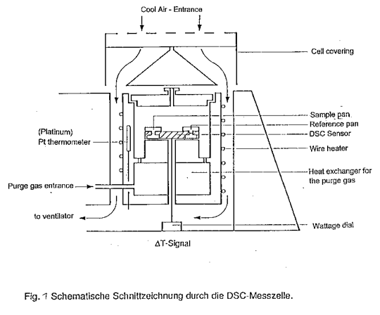
The sample to be tested and the reference material are heated at a constant rate in a gaseous environment, in our case synthetic air. The containment system for those polyolefins uses aluminum pans of 6 mm in diameter and 1.5 mm in height. The fibers are cut to small pieces of about 1 mm in length, put into the pan and covered by a perforated lid. Through special electronic configuration of the apparatus, the temperatures of the sample and reference pans will be held at the same value. Now the temperatures of both sample pans will increase with constant velocity. If a heat gradient appears, for example through a melting event of the fiber material, then additional heat, in the form of electrical energy, must be supplied to the pan. This additional heat is the melting heat which is visible in the corresponding peak on the DCS Graph.
Our experiments are carried out with the a METTLER device TA 4000.
(METTLER TA 4000/TC11/DSC 30.)
3. PRINCIPAL CHARACTERISTICS OF POLYMER DSC-ANALYSIS OF POLYOLEFINS
With the help of DSC it is often possible to make a very quick identification of a polymer. Let's begin with the simplest example, the polyethylene homopolymer.
Figure 2 : Melting and Oxidation of Polyethylen in air
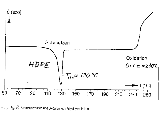
Here you see, for example, a characteristic Graph. At 130°C one can see the endothermic melting peak, and from this we can conclude that it is HDPE. The exothermic oxidation begins at about 230 °C. The slope of the curve is a means for measuring for the speed of oxidation. Exothermal oxidation is signalled normally by an abrupt increase in the specimen's evolved heat. The oxidation induction temperature (OITE) will increase with better stabilization.
Figure 3 : Melting of a Polyethylene / Polypropylene Blend
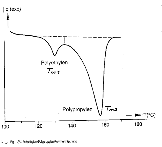
Here you can see a typical graph of a polyethylene-polypropylene blend, that means a mixture of both polymers.
In the area of 130 °C the PE component begins to melt, while the PP component melts at about 157°C.
In conjunction with these both graphs we can illustrate the most important parameters and dimensions of such an experiment:
Table 2: Parameters and results of special DSC-experiments
| Test portion | ca. 10 mg | |
| Purge gas | synthetic air | |
| Rate of heating | 10 °C / min | |
| Melting point of 1st component | Tm1 | °C |
| Melting point of 2nd component | Tm2 | °C |
| Melting heat of 1st component | D H1 | J/g |
| Melting heat of 2nd component | D H2 | J/g |
| Oxidation Induction Temperature | OITE | °C |
| Slope at OITE | Slope | W/gK |
The abbreviation OITE is used here in order to avoid confusion with OIT defined above by ASTM D 3895-95.
All marled items can be measured by DSC an can be used for identification of the fiebre material.
One should not view these Graphs as a comprehensive analysis of the material by any means, but rather as means of identification. For example, if the product "Turf 95" gave a graph with certain values of those six parameters, and two years later the product is shown to give the same Graph, then it is very probable that there has been no change in the composition of the fibers. Should complete material analysis be necessary, there are always spectrometry or chromatography methods that can be used in our institute.
4. SOME REMARKS ON POLYMER STRUCTURE
For better interpretation of the DSC graphs it seems to be useful to remember the structure of polymer molecules.
Figure 4: Thermoplastics
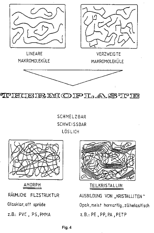
Thermoplastics can have very different molecule structures. As a matter of principle, one usually distinguishes between linear and branched molecules, and both can form amorphous or semicrystalline polymers. Examples for amorphous thermoplastics are PS and PVC, those for semicrystalline thermoplastics are PE, PP and PA.
Amorphous thermoplastics do not have a distinct melting point. When heated, they begin to gradually soften as they approach the Glass transition temperature.
However, semicrystalline thermoplastics have shown a very pronounced melting scheme in a relatively small temperature area. The entire melting process is characteristic for every plastic; that results in a special position and shape of the melting peak, which are for example different for PP and PE. Nevertheless, different PE structures vary as well. For example HDPE shows a Tm of 130 °C, whereas the Tm value of LDPE is around 120 °C.
Figure 5: Molecular structure of PE und PP
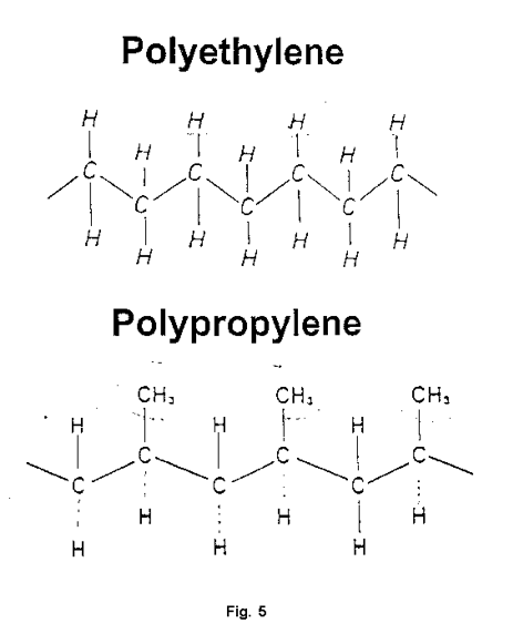
This figure shows as a refresher (as an aid) schematically the structure of single PE- and PP-molecules.
Figure 6: Different PE-types
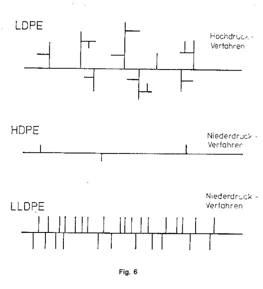
Here we can see three different individual PE-molecules. According to the specific procedure of polymerization we get a completely different architecture. It is easy to understand, that the linear molecules of HDPE will form greater crystalline zones then the other two types of molecules shown here. Therefore HDPE also shows the highest melting heat.
Whenever we have pure PE or PP, i.e. homopolymers, the DSC graphs are somewhat easy to interprete. If we have however combinations of those components, it can become quite difficult. And such a combination is made to improve flexibility and impact resistance of PP. Then we succeed in lowering the Glass Tranistion Temperature from around -5 °C to about -20 °C and to make the material flexible also at low temperatures. One can also use this for pole fibers for synthetic turf. The addition of PE to PP should improve the fibers in regards to malleability, smoothness and abrasion.
Fundamentally, there are two means in which to combine polymers with one another:
1) Through mixing the two polymers or
2) Through copolymerization.
Generally mixing two polymers produces two phases, in which one phase, composed more or less of bigger particles, is embedded into the matrix of the other. Consequently, the two polymers have considerably independent melting points, which can be easily interpreted.
Figure 7: Molecular structure of Copolymerisates
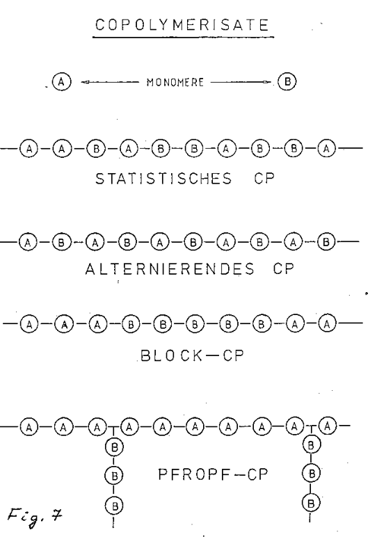
For most uses copolymerisation is the better way to combine two different components, at least as polyolefins are concerned. In this figure you can see the principle of how two different monomers can be combined to form a macromolecule. According to the specific type of polymerisation (which is determined by the catalyst system), we can produce different kinds of copolymers:
random, alternating, sequential or graft copolymers. We can understand quite easily that a random copolymer, consisting of 40% ethylen and 60 % propylen monomers, for example, cannot form crystalline zones which are characteristic for PE or PP. Therefore the DSC Analysis will not show the melting peaks of PE or PP. Nevertheless, a graft polymer with a main chain (backbone) of PP and only a few short grafted PE-side chains would show the PP-Peak at around 160 °C but no PE-Peak.
5. DISCUSSION OF RESULTS OF DSC-ANALYSIS FROM ARTIFICIAL TURF FIBRES
After this excursion to the basics of polymers some example of fibre analysis:
Figure 8: DSC Graph Nr. 1 of fibres consisting of PP
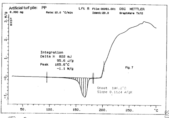
Here you see a DSC-graph of a PP-Fibre. There is no PE-Peak in the region around 125 °C but only a PP peak around 165 °C. The melting heat ist about 96 J/g. The oxidative degradation is starting at an OITE of about 196 °C.
Figure 9: DSC Graph Nr. 2 of fibres consisting of PP
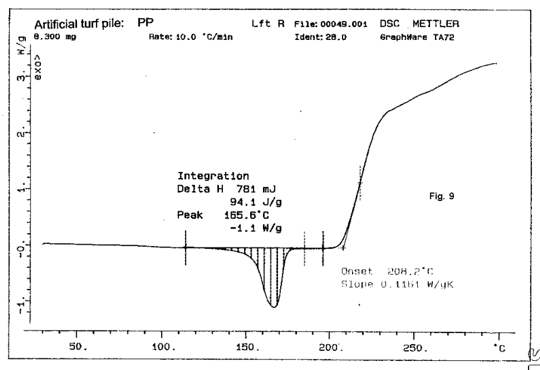
Here you can see another DSC-graph of a PP-Fibre with almost the same peak around 165 °C and almost the same melting heat. But the OITE-value is 12 °C higher, namely 208 °C. This means another - probably better - stabilization system against thermal oxidation. As we know, the stabilization compunds are designed as a synergistic system against thermal and UV-degradation. Therefore we can suppose that a high OITE value points to a good thermal stability and to a good UV-stability as well. Nevertheless it´s not at all a reliable proof of good UV-stability or weatherability.
Figure 10: DSC Graph Nr. 1 of fibres consisting of PP + PE
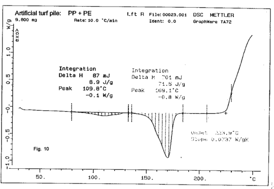
This DSC-gaph shows two peaks with maxima at about 110 °C and 169 °C, corresponding to the PE- and the PP-component. The vagueness of the PE-peak points to the copolymer type. The OITE is about 224 °C and thus by far higher than the values discussed already. These results are in accordance with the good artificial weathering resistance found in laboratory testing.
Figure 11: DSC Graph Nr. 2 of fibres consisting of PP + PE
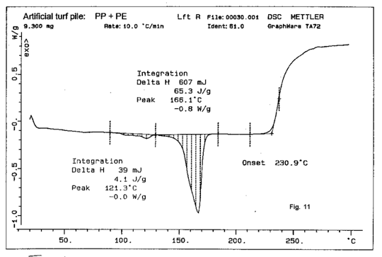
There you can see the DSC-graph of another PP/PE-copolymer with a somewhat different characteristic, but as a whole quite similar to the last DSC-graph. Also, here we can find no sharp and pronounced PE-peak.
In both polymers PP is the dominating component and seems clearly to form the main chain of every single molecule.
Figure 12: DSC Graph of fibres consisting of PE + PP
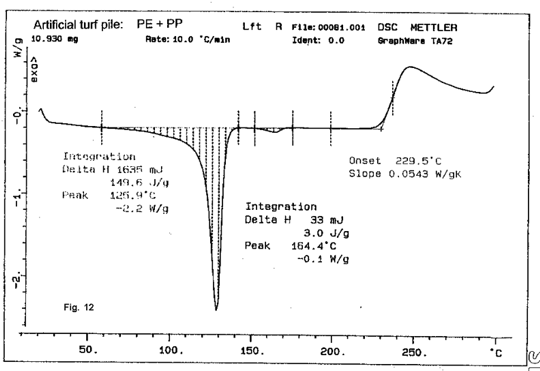
This graph shows a completely other characteristic, namely a sharp and pronounced PE-peak at about 130 °C and a very small PP-peak at 164 °C. That probably means a main chain of PE with few and possibly short PP grafted side chains. Furthermore the melting heat of PE of about 150 J/g seems quite striking. For the great PP-peaks in the graphs discussed before we had found just about 95 J/g. This is in accordance with the well known difference of the melting heats for the pure homopolymers HDPE and PP.
(the melting point of HDPE can be up to 135 °C)
Figure 13: DSC Graph of PP-pipe material - measurement of OIT
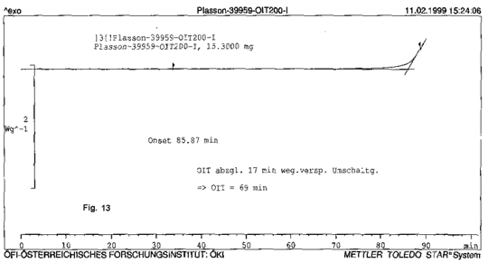
Finally here a special DSC-graph, which shows the measurement of the OIT for a PE pipe resin, according to the ASTM resp. EN-standard I mentioned already. OIT: that means OXIDATION INDUCTION TIME and not TEMPERATURE. In this experiment, the sample is heated rapidly to 200 °C and subsequently held at that constant temperature in oxygen atmosphere. So it is an isothermal experiment where we have to wait until the exothermal oxidation starts. This time is called OIT and is normally characteristic for the effectiveness of the stabilization system against thermal degredation.
Of course the question arrives why we have not stayed at OIT but changed to OITE. The answer ist very simple: it was for practical reasons. When I measure OITE then I have a terminated time program, where I get my results and this is important for varying polymer material as we find it in turf fibres. The OIT-measurements on turf fibres have shown very widely differing results, so that it would cost too much time to survey.
References
1) ASTM D 3895 - 95: Oxidative-Induction Time of Polyolefins by Differential Scanning Calorimetry
2) EN 728: Plastics piping and ducting systems - Polyolefin pipes and fittings
3) Turi, Edith A.: Thermal Characterization of Polymeric Materials , Volume 1 ,
Academic Press San Diego ..... Toronto 1997, 1981 (eb. ?) about 1400 pages.
Volume 2: 1000 pages.
Lausanne: 28 & 29 November 2024
The ISSS has successfully concluded the AGM and the Technical Conference in Lausanne. Scientific and Individual Members present accepted financials, audit report and activity schedule as presented.
Details Here